Understanding Production Factor Markets: Labor, Capital, and Land

The production of a good (or service provision) requires the use of certain resources.

The main resources are labor, capital and land.

Capital includes machinery, infrastructure, buildings, etc., which means any element that the company’s fixed assets manufactured by man, and as such is used in the production process.

When a company needs a factor of production goes to their respective markets to purchase.

In each of these markets for productive factors there is a supply and demand which determine a breakeven point (cut point of the curves). These markets have similar performances so we’ll look at just one, that of labor.

In this analysis we assume that both markets of different factors such as the company develops products that are perfectly competitive.

This factor of production is priced on the market that is wages.

When a firm hiring labor studies performed a comparative study of employee benefit that can generate versus the cost that is going to cost.

This benefit can be obtained by going to the production function:

The production function relates the output produced with the volume used by a particular factor of production (other factors held constant).

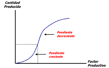
The slope of this curve represents the increase in output that is obtained by increasing the productive factor in a unit.

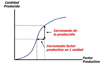
The slope of this curve is decreasing due to the law of diminishing returns.

As new workers are entering the production increase obtained is diminishing.

Therefore, the production value that provides an additional worker will be increasingly marginalized.

The first worker will contribute more than the second, the second the third, and so on.

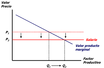
The company will hire as long as the value that the new employee is greater than the salary that you must pay.

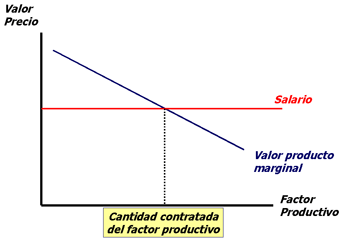
The company contracted to the point of cutting the wage line and the curve of the value contributed by the new employee (equilibrium point).

To the left of that point you should keep hiring as the value contributed by each new employee is higher than his salary.

To the right of that point is just the opposite: the worker’s wage is higher than the value of output it generates.

The level of output the firm gets contract the volume of productive factors that determines the cutoff point coincides with the point that determines the competitive market equilibrium (cutoff value of marginal revenue and marginal cost).

Let us consider the purposes of simplicity that labor is the only production factor used by an enterprise.

At point A the chart above is satisfied that:

Marginal production value = Salary

Substituting the “marginal value of production” for its formula we get:

Price * Production marginal = Salary

Turning the term “marginal production volume” on the other side of the equation:

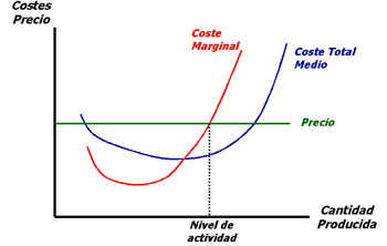
Price = Salary / marginal production volume

The right part of the equation is equal to marginal cost, cost incurred when production is increased by one unit (we are considering that salary is the only cost).

Therefore:

Price = Marginal Cost

That is precisely the equality is satisfied in equilibrium.

The previous equality shows the relationship between market factors and the supply function of a company:

The company employs inputs until the value of additional output is equal to the cost factor. This level of production corresponds to the point where marginal revenue equals marginal cost.

There is a direct relationship between declining marginal product of inputs and increasing marginal cost of production function.

Any movement in supply or demand for a factor alter its equilibrium price.

A shift in supply or demand of workers affected by both the equilibrium wage.

This variation of wages in turn changed the amount of this factor demanded by the company.

The firm labor demand until the wage equals the marginal value product.

Therefore, if the salary ranges also vary the value of marginal product because at the point of market equilibrium factors both variables must match.

An example:

The labor supply curve shifts to the right by strong immigration. The new equilibrium involves much hired labor and lower wage.

By increasing labor lowers the marginal product (law of diminishing returns) which implies a lower marginal value product.

Salary and marginal value product is cut into a new point in which both variables decreased.

Another example:

The labor demand curve shifts to the right (for example, strong demand for computers require the industry to recruit more manpower).

The rightward shift of the demand curve increases the equilibrium wage.

Alongside the demand for computers raises its prices, so the marginal value product of an additional worker increases.

The productivity of each factor will depend on the available volume of the other factors.

For example, the productivity of a field worker is related to the greater or lesser availability of machinery.

Variations in the amount of available factor (displacement of its equilibrium point by movements in supply or demand) affect the price of that factor but also the price of all other factors.

Since the price of each factor will depend on their productivity and this relates to the availability of other factors.

For example, increasing the manpower available for the field that their wages will vary, but at the same time this increased availability of labor will increase the productivity of land and therefore so will the price of this factor.