Descriptive and Inferential Statistics: A Comprehensive Guide

Posted on May 13, 2024 in Mathematics

Lecture 10: Distributions and Descriptive Statistics

Distinguish between raw data, dataset, statistics

• Raw data: Numerical data collected from each participant
  Dataset: Collection of the raw data for the same variables for a set of participants

• Statistics: Any numerical indicator of a set of data

Distinguish between descriptive and inferential statistics and identify the purpose of each

• Descriptive Statistics: Simple descriptions about the characteristics of a set of quantitative data. Convey essential information about the data as a whole
  Measures of Central Tendency and Measures of Variability

• Inferential Statistics: Allow us to draw conclusions about the population of interest via the sample of participants. Allow us to understand relationships between variables

Normal distribution – definition and properties

• A theoretical distribution of scores in which one side of the curve is a mirror image of the other

• Horizontal Axis: All possible values for the variable

• Vertical Axis: Relative frequency at which values occur

• In a perfect bell curve, the mean, median, and mode all have the same value.

• In a perfect bell curve, the mean, median, and mode all have the same value.

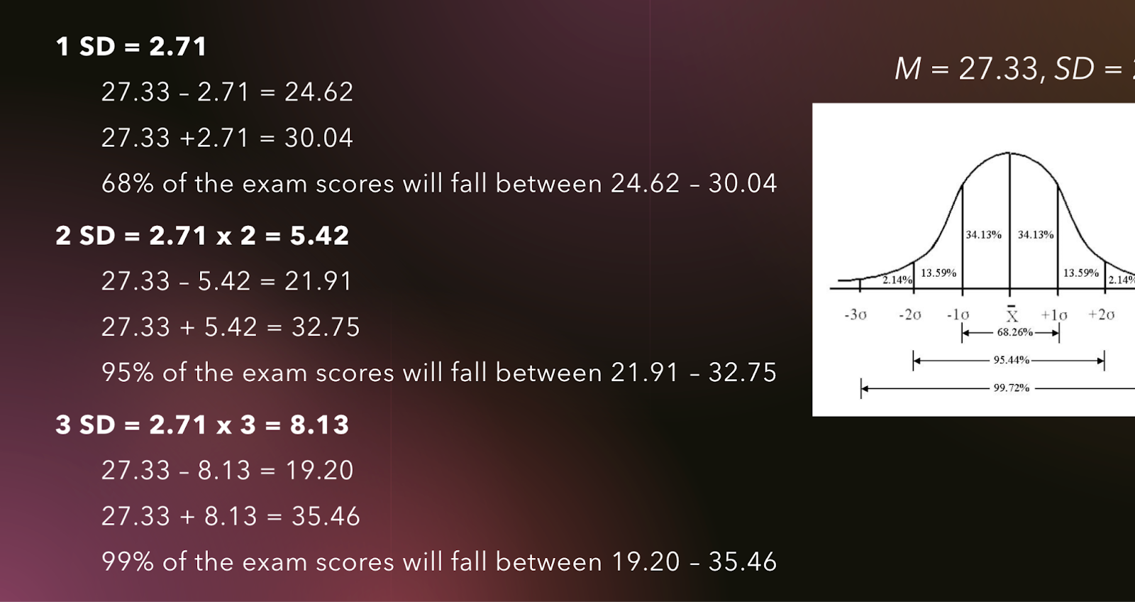
• ~68% of the distribution falls within one standard deviation from the mean

• ~95% of the distributions falls within two standard deviations from the mean

•  ~99% of the distribution falls within three standard deviations from the mean

Skew – general definition- 

A measure of non-symmetry in distributions, deviation from normality

• When distributions are skewed, the scores within that distribution are piled up on one end more than the other
  The direction of the skew (positive or negative) is indicated by the thin part, or tail, not the end where the numbers pile up

Positive and Negative skew – definitions, properties, examples

• Positive skew: few scores on the right side of the curve
  • Mean > Median
  • Few extremely high scores
  Points to the right

•  Negative skew: few scores on the left side of the curve
  • Mean

• When distributions are skewed, the median is a better measure of central tendency

E.g., when is the mean > the mode? Which side does the tail point?

Answered above

Kurtosis – general definition- measure of the tailedness of a distribution

1. Platykurtic and leptokurtic – definitions, properties, examples

Platykurtic

• Definition: A distribution is relatively flat. Scores cluster less tightly around the mean

• Properties: Indicates that the distribution has lighter tails and is less peaked compared to a normal distribution.

• Example: Exam scores where most students scored around the median, with very few very high or very low scores, suggesting a broad spread of results without extreme outliers.

Leptokurtic

• Definition: A distribution is relatively peaked. Scores cluster tightly around the mean

• Properties: Indicates that the distribution has heavier tails and is more sharply peaked than a normal distribution.

• Example: An exam with a majority of the scores clustered around a high or low average, but also with some extremely high or low scores, resulting in significant outliers on both ends.

Types of descriptive statistics

Frequencies

• Definition: Number of cases for each category of the variable.

• Calculation: Count how many times each category or value appears.

Measures of central tendency – mean, median, mode

• Mean- add all and divide by N

• Median-Middle

• Mode-Score that appears most often in the dataset

Conceptual and statistical definitions, how to determine/calculate, and utility in describing a dataset

Measures of variability – range, variance, standard deviation

• Range- Distance between lowest and highest value in a distribution

• Deviation =X-MEAN ALL OF EM

• Sum of Squares- Sum of the squared deviation scores
  
  

• Variance- Sum of Squares divided by N (when u add the sum of all the squared numbers divide by N)

• Standard Deviation-Square root of the variance

1. Conceptual and statistical definitions, how to determine/calculate, and utility in describing a datasetx

Lecture 11: Inferential Statistics

Definition of inferential statistics and their purpose (i.e., estimating the population parameters from a given sample)

• Def: Statistical procedures that allow researchers to go beyond the sample and make statements about the population via data gathered from the sample

3 types of distributions: population, sample, sampling

• Population: Frequency with which cases that make up a population are arranged ▪ Parameters: Mean, Median, Mode, SD

• Sample Distribution: Frequency with which cases that make up a sample are arranged ▪ Statistics: Mean, Median, Mode, SD

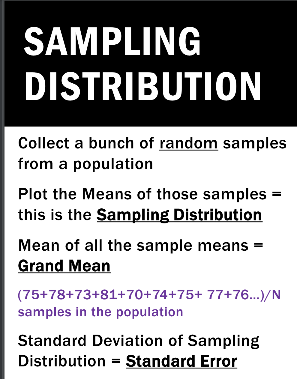
• Sampling Distribution: Frequency with which values of statistics are observed or expected to be observed when numerous random samples are drawn from a given population

Central Limit Theorem, including:

Primary assumptions

• Random Sampling: Samples must be drawn at random from the population.

• Sample Size: Larger sample sizes (typically n > 30) are more likely to produce a sample mean that is normally distributed around the population mean, regardless of the population’s distribution

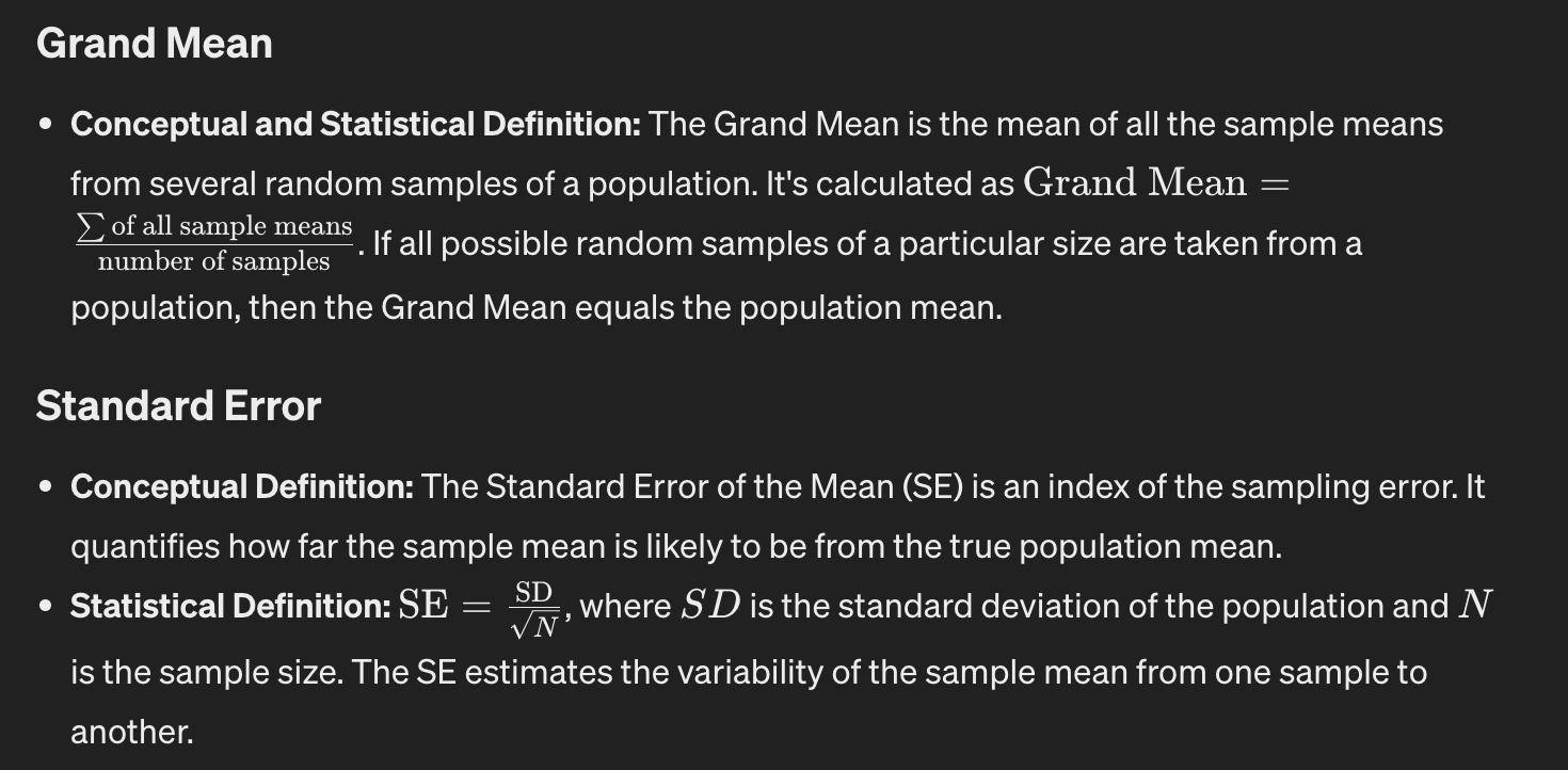
1. Grand Mean and Standard Error – conceptual and statistical definitions

Hypothesis testing and significance levels

• When we put forth a research hypothesis, we are actually testing the null hypothesis. We believe in the null hypothesis until we have enough evidence to show it isn’t true 

Definition of significance level (p-value) and how to interpret p-values

• The level of error a researcher is willing to accept for a given statistical test

•  p

• To reject the null hypothesis, we must conclude that the probability level of our statistical test is less than .05

The 7 steps of significance testing – you will need to know these steps for all inferential statistics calculations

• 1. State a research hypothesis and its null hypothesis

•  2. “Decide” on a p-value. a) We will always use p

• 3. Confirm appropriate statistical test. 

• 4. Compute the test statistic. a) This is derived from a formula (e.g., correlation) b) Use the absolute value.

• 5. Determine the critical value.

  •  a) This is the minimum point of significance – creates Region of Rejection and Region of Acceptance 

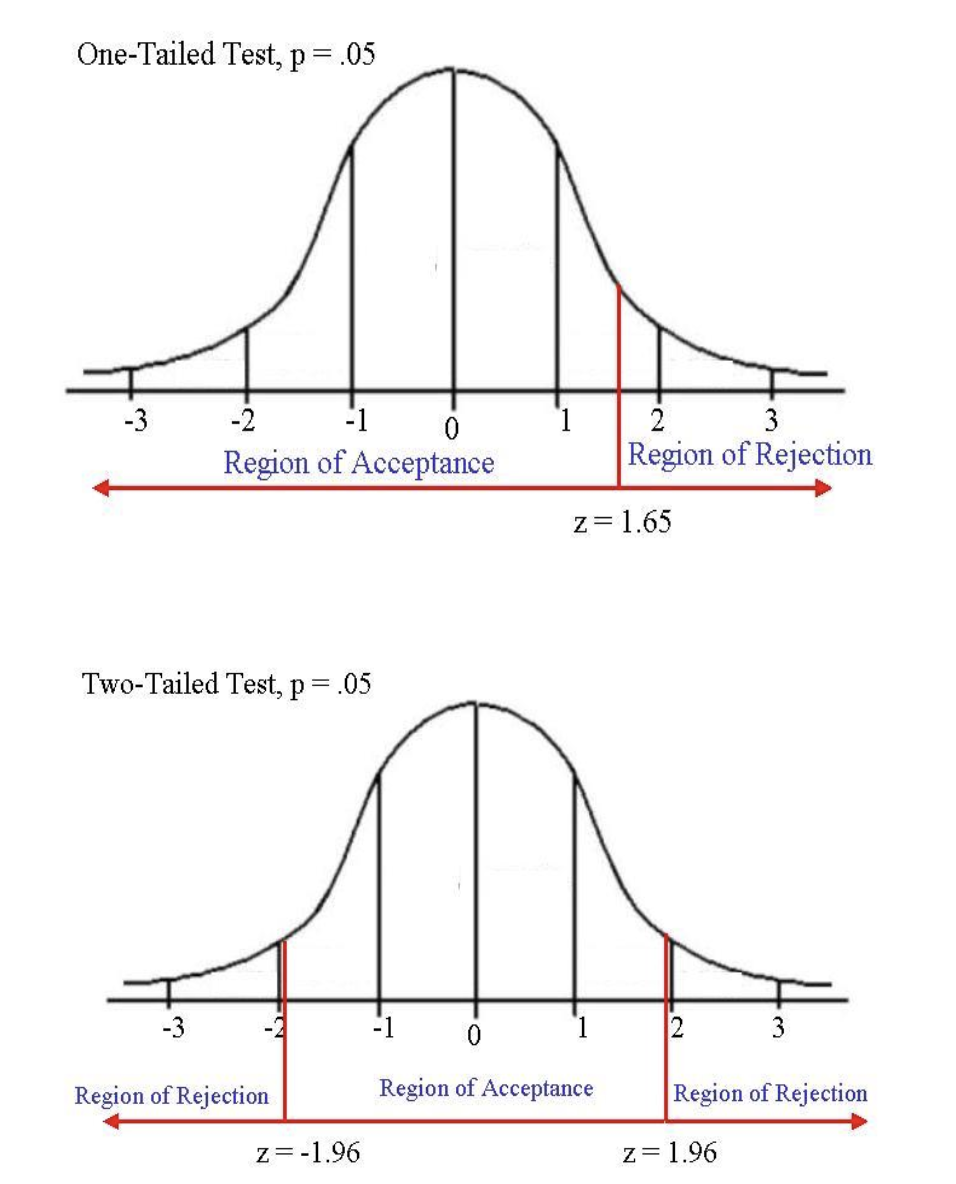
  • b) Must determine if the test is one-tailed or two-tailed i. Directional or Non-directional hypothesis 

  • c) Must calculate degrees of freedom 

    • N1+N2-2

  • d) Critical value is derived from a table We will discuss these later!

• 6. Compare the (absolute value of the) test statistic to the critical value. 

  • a) If the (absolute value of the) test statistic (TS) is greater than the critical value (CV), the test is significant. 

• 7. Accept or reject the null hypothesis.

  • a) Accept null hypothesis if CV > TS

  •  b) Reject null hypothesis if CV

Directional vs. Non-directional hypotheses and how they influence rejection or acceptance of the null and research hypotheses

• Directional Hypotheses Region of rejection on one side of the distribution, based on critical value 

• Non-Directional Hypotheses Region of rejection divided onto both sides of the distribution, based on critical value

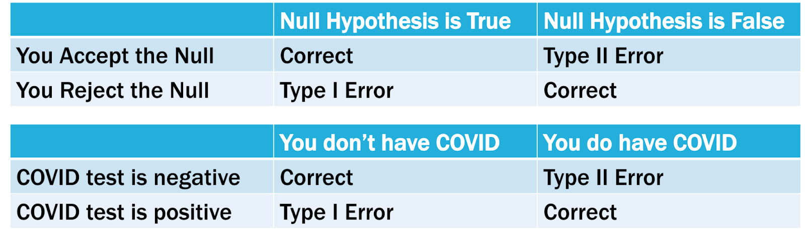
Type I and Type II Errors – when they occur, the relationship between them, and how to protect against them

Lecture 12: Independent and Dependent Samples t-tests

Distinguish between independent and dependent samples tests

• Independent-Measures whether the 2 groups of the IV are significantly different in terms of their scores on the DV

• Dependent-Measures participants’ change in DV scores from Time 1 to Time 2

The purpose of the independent and dependent samples tests

• Independent-Measures whether two groups differentiated by an independent variable (IV) are significantly different in terms of their scores on a dependent variable (DV). This test is used when each group contains a different set of sampled units, which are selected independently of each other.

• Dependent-Measures changes in the dependent variable (DV) scores from one time point to another within the same participants. This test is suitable for longitudinal designs, such as pre-test and post-test setups, to see if the DV scores of the same participants are significantly different at two time points.

]

Conceptual and statistical definitions of independent samples test

• This test is used to determine if there are differences between two groups on a continuous dependent variable, where the groups are formed based on a categorical independent variable. It is specifically applicable when each group consists of different individuals who are not related or matched in any way, ensuring that the samples are independent of each other.

• Statistical Definition: The independent samples t-test compares the means of two independent groups in order to determine whether there is statistical evidence that the associated population means are significantly different. The test calculates a t-value using the formula:

Type of data required to perform the independent samples test (e.g., the level of measurement for each variable) and examples

• Independent Variable (IV): Must be categorical, comprising exactly two groups. This variable classifies the sample into two distinct groups.

• Dependent Variable (DV): Must be continuous, which implies it is measured at the interval or ratio level. The DV is the variable tested to see if there are differences between the two groups.

Identify the independent and dependent samples tests from a given hypothesis/RQ and variable measure description

LOok UP

Formulas will be provided in a matching section, but you still need to know how to conduct the independent samples t-test calculation (e.g., the steps involved and the application of the formula), how to find the critical value from a table provided, how to report the result, and whether or not the research hypothesis proposed is supported

• Null Hypothesis: The 2 groups are not significantly different in terms of the DV

• Research Hypothesis: The 2 groups are significantlydifferent

We accept the null hypothesis. The research hypothesis is not supported: participants who received positive feedback did not answer significantly more questions correctly than those who received negative feedback.

• One-tailed t-test: Use this when the hypothesis specifies a direction of the effect, such as expecting one group to perform better or worse than another based on the independent variable.

• Two-tailed t-test: Use this when the hypothesis does not specify a direction and only indicates that there will be a difference between the groups, without stating which direction the difference will be.

• State the Research Hypothesis and Null Hypothesis.

  • Identify and clearly define both the research hypothesis (HR) and the null hypothesis (H0).

• Decide on a p-value.

  • Determine the level of significance, commonly set at p

• Confirm the Appropriate Statistical Test.

  • Verify that the t-test is suitable for the data and research question.

• Calculate the Test Statistics.

  • Use the t-test formula to calculate the t-value.

• Determine the Critical Value.

  • Calculate the degrees of freedom and refer to a t-distribution table to find the critical value, based on whether the test is one-tailed or two-tailed.

• Compare the Test Statistic to the Critical Value.

  • Compare the calculated t-value to the critical value to determine whether to reject or accept the null hypothesis.

• Accept or Reject the Null Hypothesis.

  • Based on the comparison, decide whether the results support rejecting the null hypothesis in favor of the research hypothesis, or not.

Lecture 13: Correlations

Conceptual and statistical definitions, including positive and negative correlations

Conceptual Definitions

• Correlation: A statistical measure that expresses the extent to which two variables are linearly related. It’s a way to examine whether changes in one variable correspond to changes in another variable.

Statistical Definitions

• Correlation Coefficient (r): A numerical index that ranges from -1.0 to +1.0. It measures the degree of linear association between two continuous variables. The correlation coefficient is always a decimal value.

Positive Correlation

• Conceptual Definition: Occurs when increases in one variable are associated with increases in another variable, or decreases in one variable are associated with decreases in another. This means that the variables move in the same direction.

• Statistical Indicator: Indicated by a positive number (r > 0). For example, a correlation coefficient of +0.70 suggests a strong positive correlation.

Negative (Inverse) Correlation

• Conceptual Definition: Occurs when increases in one variable are associated with decreases in another variable, and vice versa. This means that the variables move in opposite directions.

• Statistical Indicator: Indicated by a negative number (r

The strength of the relationship as indicated by the r-value

• The r-value (correlation coefficient) refers to the strength of the relationship between the two variables of interest.

• To determine a correlation’s strength, examine its absolute value:

  • >.90: Very strong

  • .70 – .90: Strong

  • .40 – .70: Moderate

  • .20 – .40: Weak

  • 
    

The coefficient of determination, how to compute it, and what it means

• Conceptual Definition: The coefficient of determination, expressed as R^2 , represents the percentage of the variance in one variable that is predictable from the other variable. It quantifies how well the values fit the data compared to the mean. How to Compute Calculation: To compute the coefficient of determination, square the correlation coefficient ( Formula: 𝑅^2=𝑟^2)

Type of data required to perform the test (e.g., the level of measurement for each variable) and examples

• Variables: Both variables must be continuous, measured at either the interval or ratio level. This ensures that the data can be meaningfully ordered and differences between values are consistent.

1. Positive Correlation Example:

   • TikTok Use vs. Need for Approval:

     • Variable X: TikTok use (hours per week) – continuous, ratio level.

     • Variable Y: Need for approval (measured on NFA scale score) – continuous, interval level.